journey
    title Race results
      Section Largest dAIC
        Worst model: 0
      Section Intermediate dAIC
        Next best model: 3
      Section dAIC = 0
        Best model: 6
Compare models
Delta AIC1
You can calculate a Delta AIC value for each model
Delta AIC for a model is its distance from the best model, or the information lost by moving from the best model to that model
\[ \Delta AIC_i = AIC_{model} - AIC_{best model} \]
- The best model always has Delta AIC = 0
- Smaller Delta AIC values indicate a model has more support from the data
- Larger Delta AIC values indicate more information lost, or models further from reality (your data)
Race results
Delta AIC values are like the results of a race 🏃
You compare the finish times of competitors (alternative models) with that of the winner (best model)
Compare detection functions
We’ll use the distsamp() function to analyse our data, creating a separate output object for each model1
We already have output for our half-normal null model based on the truncated water deer sightings, called hn_NullT
Let’s create a second null model using a uniform detection function:
View alternative model output
How does this output differ from the model with a half-normal detection function?
View histograms
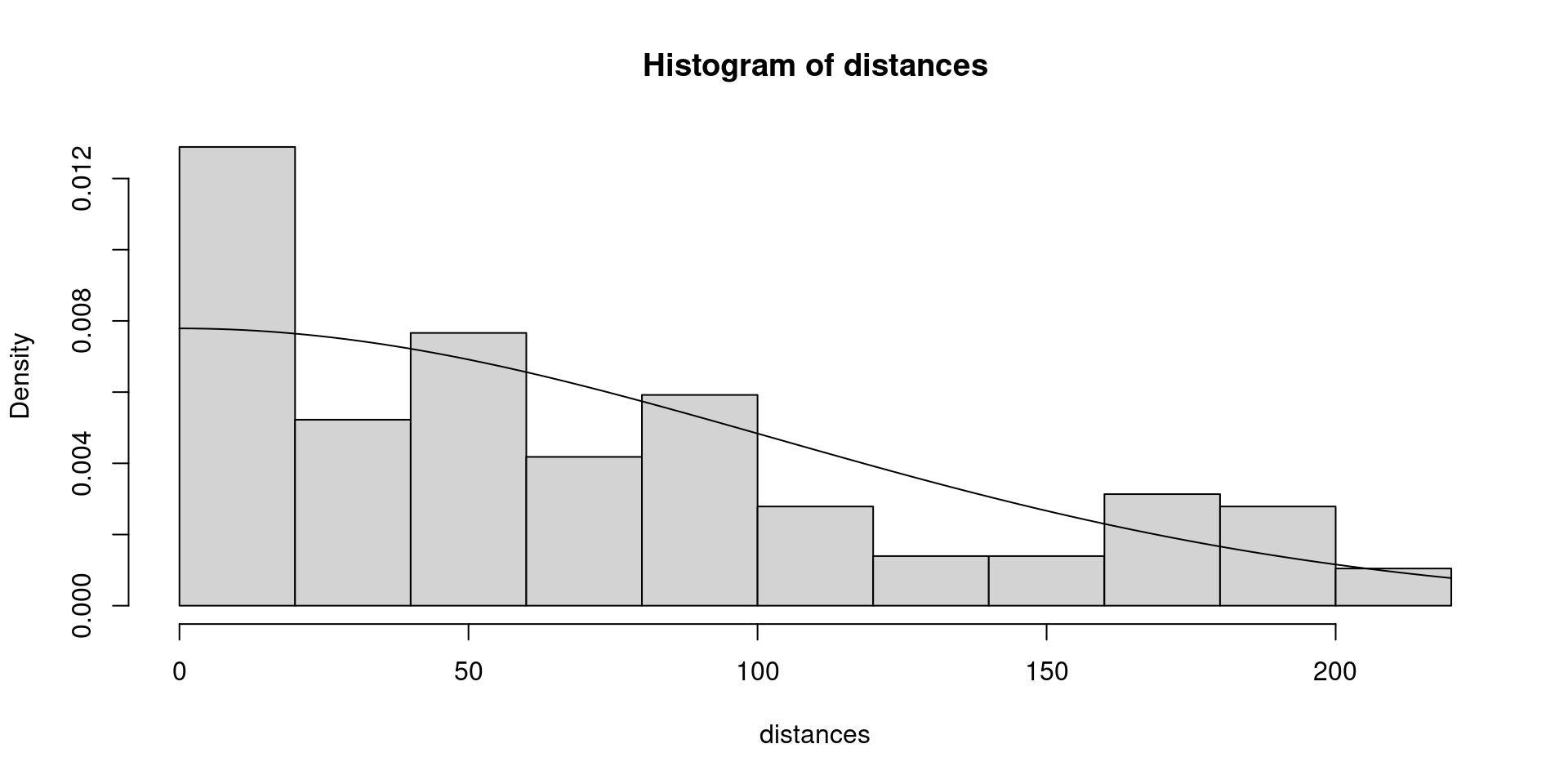
Use the hist() function to draw your detection functions over the sightings data:
Half-normal
Uniform
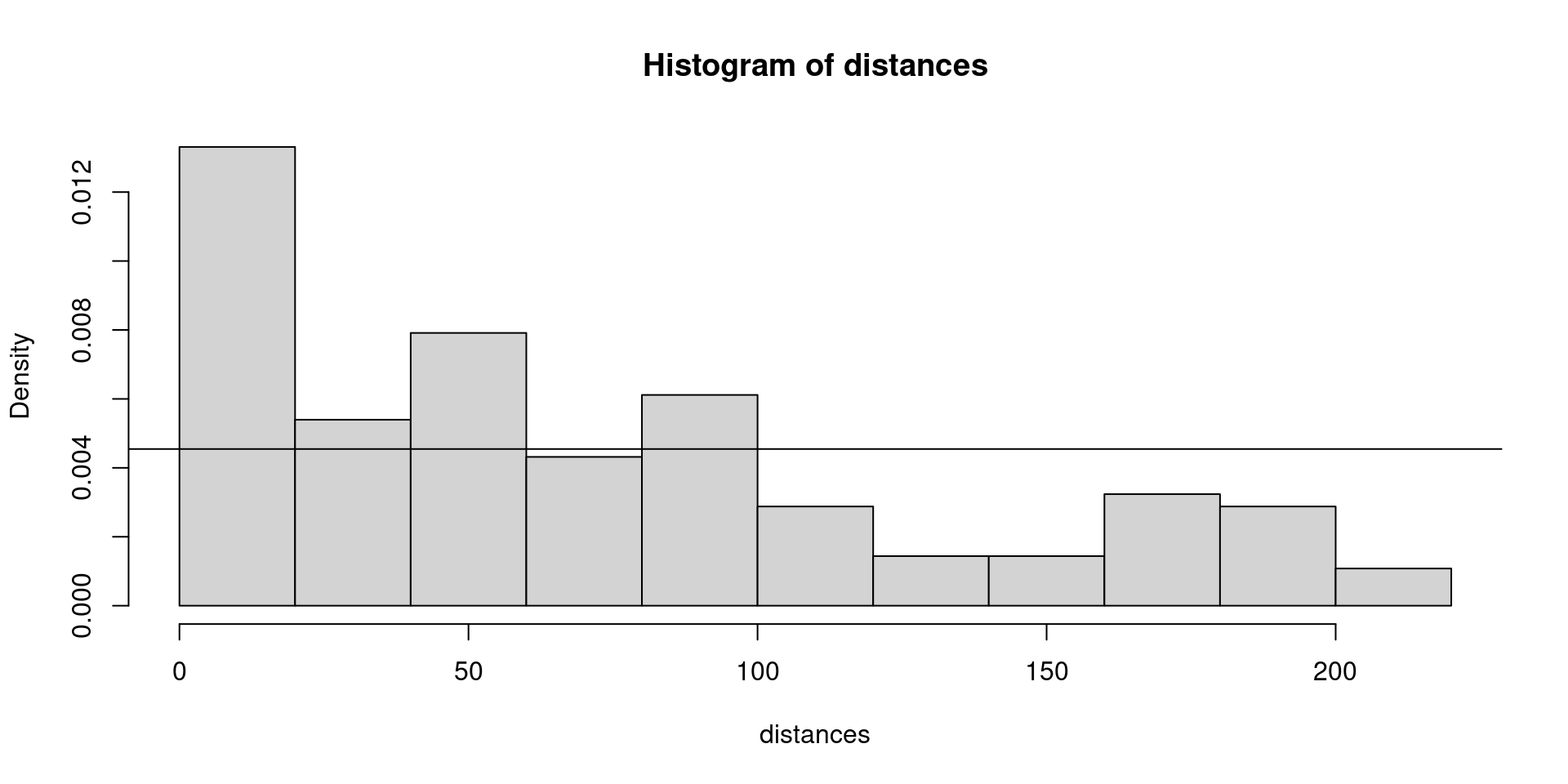
Which detection function looks like a better fit?
Next we check what the statistical support is for each detection function, using Information Theory
Create a list of models
We populate an empty list object with the results of our individual models using list()
As we create the list, we name each model so they’re easy to identify later:
- Remember that the first tilda
~in the model formula is for detection and the second is for density - We’ll use full stops
.to indicate that we’re calculating only an intercept for each parameter, rather than a covariate
We convert this standard list into a special unmarked format using fitList():
Model selection statistics
- unmarked’s
modSel()function helps us select between candidate models:
       nPars    AIC delta AICwt cumltvWt
hn..       2 361.13  0.00 1e+00     1.00
unif..     1 404.98 43.85 3e-10     1.00
R reminds us of:
- The number of parameters used to build each model
- Half-normal: 1 intercept for density + 1 for standard deviation of the half-normal curve
- Uniform model: 1 intercept for density. unmarked doesn’t implement a uniform model with a slope (straight-line decline in detectability)
- AIC, with models ordered from lowest to highest
- Delta AIC: zero is the best model, while higher \(\Delta AIC\) indicates a worse fit to our data
- Models with a higher AIC weight are better, while models with low AIC weights have little evidence to support them
Which detection function is best?
       nPars    AIC delta AICwt cumltvWt
hn..       2 361.13  0.00 1e+00     1.00
unif..     1 404.98 43.85 3e-10     1.00
Here the best-supported model is the one which uses the half-normal detection function
Its lower AIC value, dAIC of zero, and much higher AIC weight demonstrate much stronger evidence for this model than the uniform detection function
I’m sure this is no surprise, given that detection of the water deer clearly declines in a curve with distance from the transect, rather than remaining constant!
Using AIC
We don’t recommend using strict rules for dAIC values to reject models
Models with dAIC from 0 to 9 or 12 are plausible to most objective people (Anderson 2008)
- If the dAIC of a few models are close to zero, they are all strongly supported by your field data and there is little reason to choose between them
- Models with dAIC of 4-7 have less empirical support, and there is substantial evidence of a difference in fit compared to the best model
- Models with dAIC of 9-14 have relatively little support, but unless you have one clear best model, retain your entire model set and draw conclusions using model averaging
Use your understanding of the ecological system, and your judgement of the quality of your data and models