Import the data
We’ll use the read.table() function to import the transect and deer data in .csv format
Copy-paste the following code and comments into your script
Remember to edit the path to your data within here()
1 <- read.table (2 here ("data/raw_data" ,3 "DeerObs.csv" ),4 header= TRUE ,5 sep = "," )6 <- read.table (here ("data/raw_data" , "TransectLengths.csv" ), header= TRUE , sep = "," )
1
Use read.table() to import text files
2
Use here() to give the relative path within your project directory
3
Specify the file to import - the deer observations
4
First row is column headers (names)
5
Separated (Delimited) by commas - you might use tabs \t or semi-colons ; instead
6
Repeat for transect lengths
View raw data in R
In Rstudio, you should now see your DeerObs and TransectLengths objects in the Workspace (top-right)
Click on DeerObs and TransectLength to open them and check they imported correctly
Print the first few rows of each with R - it’s quicker than opening objects manually in RStudio
head (DeerObs) # print the first few rows
  TransectID Distance_m
1        T01     123.52
2        T01      37.84
3        T01     223.78
4        T01     146.80
5        T02     173.12
6        T02     189.32
  TransectID Length
1        T01   1880
2        T02   6140
3        T03  10310
4        T04  10310
5        T05  10310
6        T06  10310
Prepare data for unmarked
Before analysis, we convert our observations into the right format for unmarked
The original dataset, DeerObs.csv , contains:
🔤 The name of the transect in the first column📏 Distance to the sighted animal in the second column
unmarked expects to receive line transect data as:
A single row for each transect, with…
columns of distance intervals (distance ‘bins’, e.g. 0-20m, 20-40m etc), containing…
the number of sightings in each distance interval
We also need to specify the distance intervals we want unmarked to use. We must know our data well enough to choose:
Appropriate intervals
A sensible maximum distance
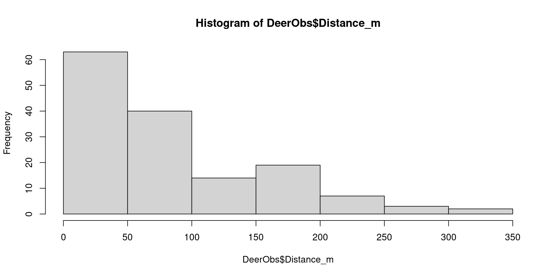
Views distances as a histogram
To help us determine appropriate intervals, plot the distances as a histogram:
hist (DeerObs$ Distance_m) # Histogram of distances to sightings
Examine the histogram to decide:
A distance interval that enables us to see the detection pattern from our surveys
Maximum distance, choosing a value which is a multiple of the interval
In this case, 25m intervals would be appropriate, and all observations are less than 350m away
Create a vector of intervals
Create a vector which describes the intervals you’ve chosen using seq()
1 <- seq (0 ,2 350 ,3 25 )
1
Create a number sequence from zero…
2
to 350…
3
in intervals of 25
[1] 0 25 50 75 100 125 150 175 200 225 250 275 300 325 350
Create an Unmarked Frame
Next we convert our re-organised deer sightings object yDat into the correct format for the unmarked package: an unmarked frame or UMF
At this stage, we provide only the deer sightings, and not any environmental covariates for transects
1 <- unmarkedFrameDS (2 y = as.matrix (yDat),3 dist.breaks = DistanceBins,4 tlength = TransectLengths$ Length,5 survey = "line" ,6 unitsIn = "m" )
1
Use unmarkedFrameDS() to create a UMF, which we call distUMF
2
Specify our dataset in matrix format, plus…
3
our distance intervals and…
4
the lengths of the transects
5
Confirm data were collected on line transect surveys (as opposed to point counts)
6
Confirm distances were measured in metres
Examine the UMF with summary()
View our new unmarked dataframe object:
head (distUMF, 3 ) # View first three rows of UMF
Data frame representation of unmarkedFrame object.
    y.1 y.2 y.3 y.4 y.5 y.6 y.7 y.8 y.9 y.10 y.11 y.12 y.13 y.14
T01   0   1   0   0   1   1   0   0   1    0    0    0    0    0
T02   4   1   3   0   2   0   3   1   0    1    1    0    0    0
T03   5   2   5   4   3   1   2   6   1    0    0    0    0    0
R has many generic functions that give different output depending on the type of input object, for example summary():
summary (distUMF) # summarise the UMF object
unmarkedFrameDS Object

line-transect survey design
Distance class cutpoints (m):  0 25 50 75 100 125 150 175 200 225 250 275 300 325 350

12 sites
Maximum number of distance classes per site: 14
Mean number of distance classes per site: 14
Sites with at least one detection: 12

Tabulation of y observations:
  0   1   2   3   4   5   6   8
108  20  19   8   5   4   3   1
Note how R summarises the number of sites (transects), as well as the number of sites with at least one detection
Examine the UMF with str()
str (distUMF) # show the structure of the UMF
Formal class 'unmarkedFrameDS' [package "unmarked"] with 9 slots
  ..@ dist.breaks: num [1:15] 0 25 50 75 100 125 150 175 200 225 ...
  ..@ tlength    : int [1:12] 1880 6140 10310 10310 10310 10310 10310 10310 10310 10310 ...
  ..@ survey     : chr "line"
  ..@ unitsIn    : chr "m"
  ..@ y          : num [1:12, 1:14] 0 4 5 3 2 3 3 8 5 0 ...
  .. ..- attr(*, "dimnames")=List of 2
  .. .. ..$ : chr [1:12] "T01" "T02" "T03" "T04" ...
  .. .. ..$ : chr [1:14] "[0,25]" "(25,50]" "(50,75]" "(75,100]" ...
  ..@ obsCovs    : NULL
  ..@ siteCovs   : NULL
  ..@ mapInfo    : NULL
  ..@ obsToY     : num [1, 1:14] 1 1 1 1 1 1 1 1 1 1 ...
R tells us:
The class of object (unmarkedFrameDS ), which is a type of list
The slots in this list, which include
The matrix of deer counts on each transect in each distance interval, y
Transect lengths, tlength
The tlength slot contains total length surveyed in metres - identical to summing the original transect lengths:
sum (distUMF@ tlength) # total transect lengthsum(TransectLengths$Length)
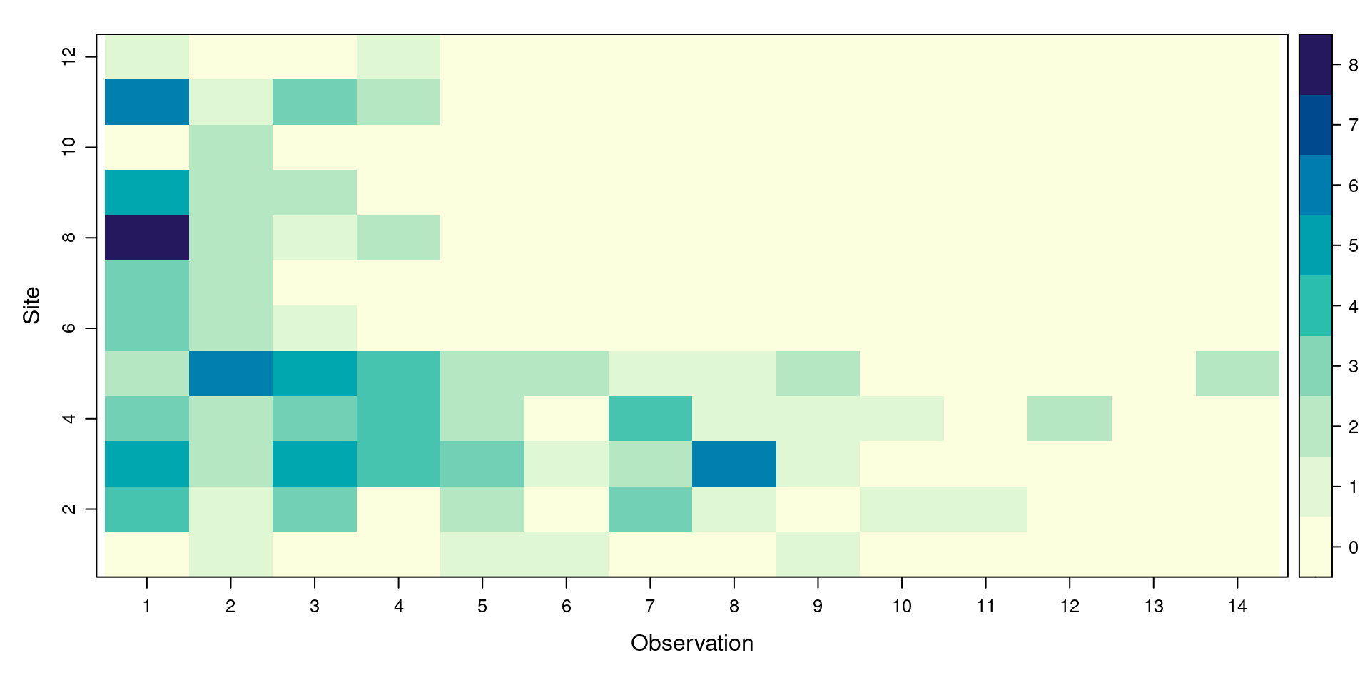
Plot the UMF
Another generic function is plot(). When used on a UMF, plot() shows us the pattern of detections on each transect (Site ) within each distance interval (Observation ):
We can also ask for information specific to UMF objects. What does this function tell us?
Calculate encounter rate
To calculate the encounter rate, divide the number of sightings by total distance surveyed
1 nrow (DeerObs) / 2 sum (distUMF@ tlength) / 3 1000 )
1
Total number of sightings
2
Total distance surveyed, in metres…
3
divided by 1000 to give us sightings per kilometre