- 1
-
Run
distsamp()and save the output as a new object called hn_Null - 2
- Our model equation - constant detection and density across transects
- 3
- Specify our UMF object
- 4
- Choose a detection function; in this case, half-normal
- 5
- Calculate density, not population size
- 6
- Units of measurement for density estimate
Run a model
The null model
The first model we’ll run is a default, or null model
The null model specifies that density and detectability are constant across the site (i.e. the same on all transects)
- This is like a null hypothesis
- Our alternative hypotheses would be that density and/or detectability vary with environmental covariates, which we cover in the Covariates module
Always include the null model
The null model is vital to include as a default in your set of models (hypotheses) to test, so you can compare more complex models with the most parsimonious (simple) model1
Detection functions
- As we discussed in Theory & applications, the way that detectability falls off with distance depends on many variables
-
Terrain ⛰️, vegetation 🌿, species size and behaviour 🐇 💨, observer expertise 👶 👵 and more
Possible detection functions:
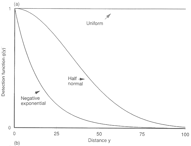
Detection function shapes
Part of our process is choosing the detection function that best fits your data
- Uniform: Most suitable for situations where detection declines only gradually with distance
- Open grassland, open water
- Half-normal: Versatile model with detection declining in a smooth curve
- Open woodlands/shrublands, undulating land
- Hazard-rate: Flexible model with a good shoulder (high detectability maintained close to the transect) before detection drops off rapidly
- Dense forest, bamboo, steep slopes or narrow valleys
A fourth model, Negative exponential, is not recommended because it crosses the y axis at a sharp angle, which means it does a poor job of modelling the area close to the transect, where you are likely to observe all animals
Run a half-normal model
We’re finally ready to run a distance sampling model! 💪
Distance sampling models two parameters simultaneously (density and detectability) rather than just one (i.e. a single response variable in a linear model)
This means that the model equation has two sections preceded by a tilde ~, for detection, and for density (in that order)
We’ll use distsamp() to run a basic model, without any covariates to explain variation in density or detectability
View model output
View a summary of your results:
Call:
distsamp(formula = ~1 ~ 1, data = distUMF, keyfun = "halfnorm",
    output = "density", unitsOut = "ha")

Density:
 Estimate    SE     z   P(>|z|)
    -2.95 0.102 -28.9 9.56e-184

Detection:
 Estimate     SE    z P(>|z|)
     4.72 0.0617 76.5       0

AIC: 381.835
This basic summary displays:
- Parameter estimates for density and detectability, on a log-scale
- Standard errors for density and detectability
- AIC value for that model1
Calculate density
Use backTransform() to convert density1 from the logistic scale:
Backtransformed linear combination(s) of Density estimate(s)

 Estimate      SE LinComb (Intercept)
   0.0523 0.00534   -2.95           1

Transformation: exp
R estimates density as 0.0523 with a standard error of 0.05
In other words, Chinese water deer occur at a density of c. 0.05 animals per hectare in this study site, equivalent to 5 deer per square kilometre
Confidence intervals
Tip
It’s always good to check the 95% confidence intervals of any parameter estimate, to see how wide they are
💡 This helps us decide how much reliance to place on our results
Use the confint() (confidence interval) function on our back-transformed value, to generate a 95% confidence interval for density of water deer:
The 95% confidence interval spans 0.043 to 0.064
Therefore, the true density of Chinese water deer might vary from 4.3 to 6.4 deer per square kilometre
Calculate detectability
Repeat the process of back-transforming parameters for detectability:
Backtransformed linear combination(s) of Detection estimate(s)

 Estimate   SE LinComb (Intercept)
      112 6.94    4.72           1

Transformation: exp 0.025 0.975
99.6304 126.896The half-normal detection function is described by a single parameter: the standard deviation of the half-normal curve
For a Normal distribution, we would expect to see 68% of the values to lie within one standard deviation from the mean, and 95% within two standard deviations
The half-normal detection function has the same properties
We can therefore expect 68% of our deer observations to be recorded within 112m of the transect, and 95% within 224m
Calculate Effective Strip Half Width
Finally, we can find out the Effective Strip Half Width (ESHW) for our deer transects
Effective Strip Half Width is the distance at which the number of animals detected beyond is equal to the number of animals undetected within it
The ESHW is equivalent to the area under the half-normal curve, from the transect line to the maximum distance we are considering, which for our deer data is 350m
Calculate ESHW by using the integrate() function:
- 1
- Integrate using the half-normal function
- 2
- From the transect line (zero metres)…
- 3
- to the maximum sighting distance
- 4
- Our estimated standard deviation
140.6611 with absolute error < 1.6e-12Effective Strip Half Width is 140m for our deer transects
Calculate detection probability
We can use Effective Strip Half Width to calculate detection probability for our water deer surveys:
Detection probability is 40%