Truncate observations

Detection function and outliers

The most informative part of the detection function is close to the y axis, i.e. estimating the value of the detection probability density function on the transect line

This is why we prefer detection function shapes like half-normal, uniform and hazard-rate, because they have a good ‘shoulder’ where detection probability is high on the transect or close by

In contrast, your field data may contain a few observations very far from the transect. These distant animals:

1. Don’t contribute much useful information
2. Can make it more difficult to model the detection function
3. May have been detected by a different process¹

1. becoming visible along a track or stream-bed, or drawing your attention with noise or unusual activity

Fitting detection functions

When you fit a detection function to your whole dataset, R may struggle to select curve parameters that fit the main dataset and the outliers

R will attempt to do this by adding more parameters to the detection function model, creating a detection function with a more complex shape

When you remove outliers, it’s easier for R to fit a simple detection function, so:

1. You calculate fewer detection parameters, meaning
2. You can include more covariates to predict density (which is what you’re really interested in!)

Right truncation

Right truncation is the step of removing distant observations

Truncation decreases the number of sightings you use, but this loss of (possibly misleading) information is outweighed by the reduced bias and increased precision of your detection function

Choose a truncation distance

There are three ways to decide which outliers to remove:

1. 👀 Look for an obvious discontinuity (gap) in the data, beyond which observations are clear outliers
2. % Remove the most distant 5-10% of your observations
3. \(g(x)\) Removing all observations for which the detection probability has fallen to 15% or below

We recommend the last approach of truncating at \(g(x) \thickapprox 0.15\) as the most effective

In practice you might use a combination of approaches to give you confidence in your choice of truncation distance

Truncate at a discontinuity

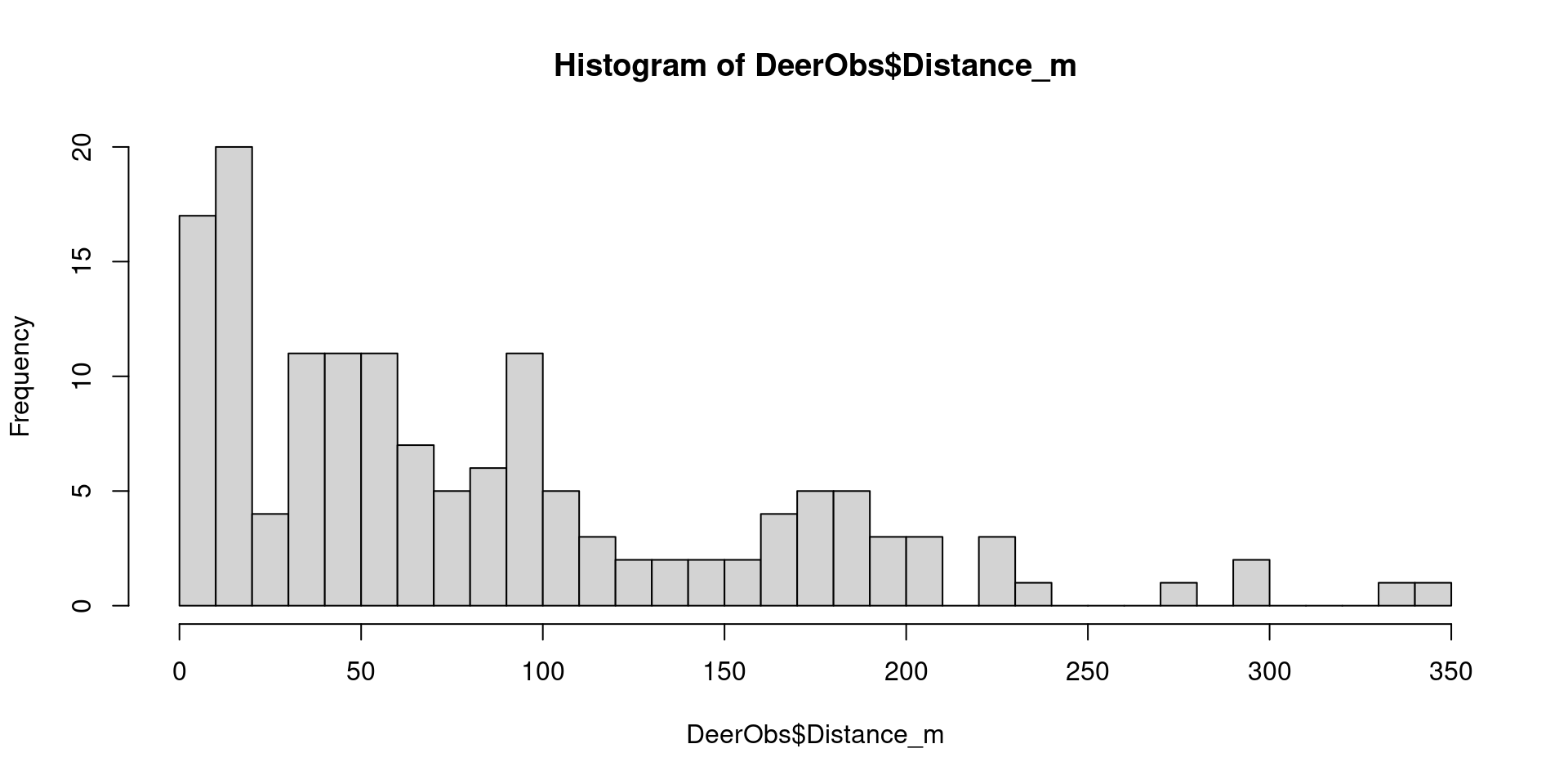
Plot a histogram of your sightings and examine it to identify gaps far from the transect:

hist(DeerObs$Distance_m,
1    breaks = seq(0,350,10))

1

Specify finer breaks to see detail (a similar plot to hist(distUMF))

What’s the first distance at which no water deer were sighted? Is there an obvious gap where it seems sensible to discard observations beyond that distance?

View raw observations

Another helpful way is to sum the distance bins from distUMF to see how sightings decline with distance from the transect

colSums(distUMF@y)

   [0,25]   (25,50]   (50,75]  (75,100] (100,125] (125,150] (150,175] (175,200] 
       40        23        23        17        10         4        10         9 
(200,225] (225,250] (250,275] (275,300] (300,325] (325,350] 
        5         2         1         2         0         2 

Choose a discontinuity

How many observations would we discard if we chose 250m, before the furthest two clusters of water deer sightings?

TruncDist250 <- 250
nrow(DeerObs[DeerObs$Distance_m > TruncDist250,]) # 5 sightings beyond 250m

[1] 5

We can take a look at the actual field data using part of the above line of code

DeerObs[DeerObs$Distance_m > TruncDist250,]

   TransectID Distance_m
7         T02     274.31
60        T04     294.07
61        T04     290.26
92        T05     332.36
95        T05     340.07

Truncate 5% of observations

The second method is to remove the most distant 5 to 10% of sightings

How many observations would you discard if you removed 5%?

1DiscardNum5 <- ceiling(nrow(DeerObs) * 0.05)
DiscardNum5

1

Multiply number of observations by 0.05 and and round up with ceiling()

[1] 8

Examine the 8 observations that would be removed

1DeerObs <- DeerObs[order(DeerObs$Distance_m),]

1

Sort our deer sightings in order of increasing distance with order()

1tail(DeerObs, n = DiscardNum5)

1

Now print to screen the observations to be discarded

   TransectID Distance_m
3         T01     223.78
59        T04     227.48
11        T02     238.38
7         T02     274.31
61        T04     290.26
60        T04     294.07
92        T05     332.36
95        T05     340.07

Truncate 10% of observations

How many observations would you discard if you removed 10%?

DiscardNum10 <- ceiling(nrow(DeerObs) * 0.1)
DiscardNum10

[1] 15

What is the furthest sighting after you’ve truncated 10% (15 sightings)?

Trunc10 <- DeerObs$Distance_m[nrow(DeerObs) - DiscardNum10]
Trunc10

[1] 189.59

Truncate at detectability < 0.15%

Run your null model first!

To truncate at \(g(x) < 0.15\), you must have already fitted a null model. We’ll use our half-normal model results from earlier

We want to estimate the distance at which detection probability has declined to 15% (\(g(x) = 0.15\))

1. Plot our model output - histogram and half-normal curve
2. Overlay a horizontal line at detection probability = 15%

Plot \(g(x) = 0.15\)

Let’s redraw our histogram, adding a horizontal dotted line to mark where detectability (y axis) falls to 15%

1hist(hn_Null)
2lines(lty = 3,
3    x = c(0,max(DistanceBins)),
4    y = c(0.15,0.15) *
5    (hist(hn_Null))$y[1])

1

Draw the histogram of deer sightings

2

Draw a dotted line

3

Specify x axis coordinates for start and end

4

Specify y axis coordinates for start and end…

5

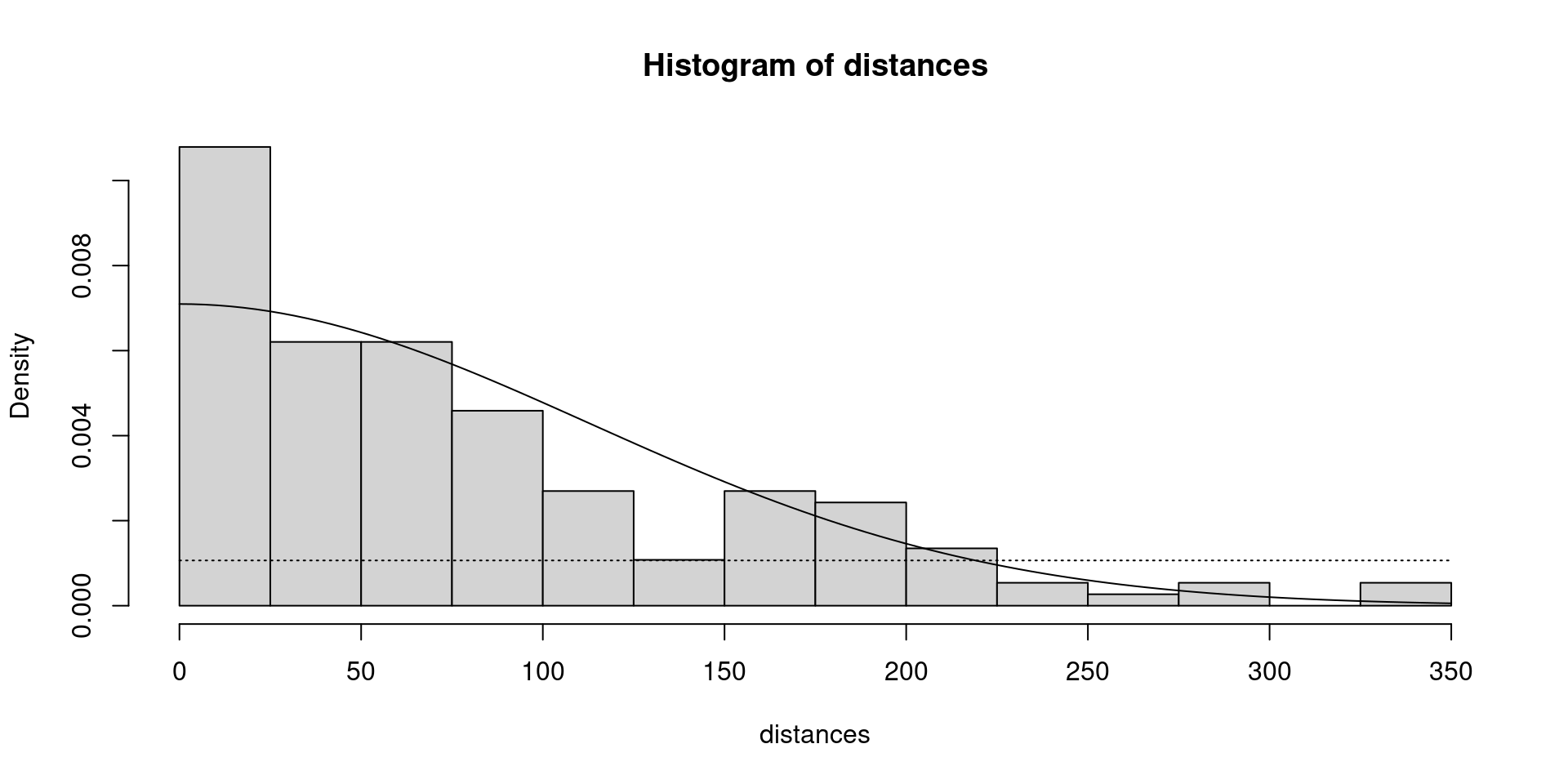
rescaled by estimated density on the transect line

Your truncation distance is the point on the x axis (distance from transect) where the half-normal model curve and the dotted line \(g(x) = 0.15\) cross

Remember that the bars are every 25m, which helps you judge the x value where our lines cross

See the next slide for our plot

Where is detectability 15%?

Sightings with detectability < 15%

In this model, detectability is 15% around 220m from the transect line

For comparison with the truncation methods above, let’s find out how many of our sightings lie beyond 220m and would be discarded based on their detection probability being less than 15%

TruncDist <- 220
nrow(DeerObs[DeerObs$Distance_m > TruncDist,]) # 9 observations

[1] 9

Using \(g(x) = 0.15\) is the most robust method for choosing a truncation distance

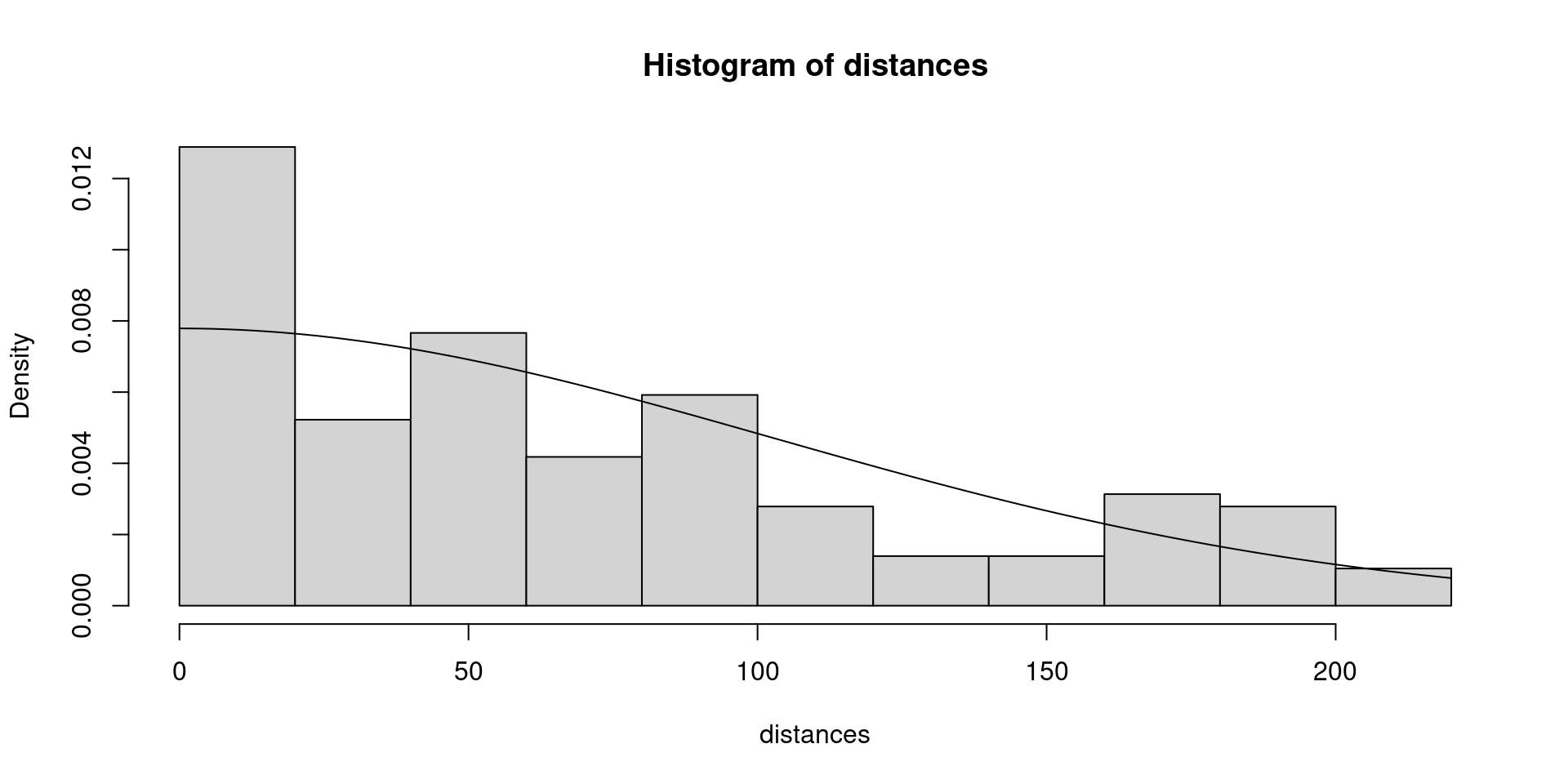
Run model on truncated data

Let’s truncate at 220m, as this lies in the middle of the distances suggested by visual discontinuities (250m) and removing 5% (222m) or 10% (190m) of observations

We need to:

1. Truncate the water deer dataset
2. Create a new UMF
3. Use the new UMF as input for a null model with a half-normal detection function

Create a new, truncated dataset:

DeerObsTrunc <- DeerObs[DeerObs$Distance_m <= TruncDist,] # Selecting obs within 220m

Create a new set of distance intervals, with a maximum of 220m:

TruncDistBins <- seq(0,TruncDist,20)

Create a truncated UMF

Format the subset of deer observations for conversion into a UMF:

TruncyDat <- formatDistData(DeerObsTrunc, # Truncated dataset
    distCol="Distance_m", # Distances
    transectNameCol="TransectID", # Transects
    dist.breaks = TruncDistBins) # Distance intervals

Convert into a UMF and examine to check all looks good:

TruncUMF <- unmarkedFrameDS(y = as.matrix(TruncyDat),
    dist.breaks = TruncDistBins,
    tlength = TransectLengths$Length,
    survey = "line",
    unitsIn = "m")
summary(TruncUMF)

unmarkedFrameDS Object

line-transect survey design
Distance class cutpoints (m):  0 20 40 60 80 100 120 140 160 180 200 220 

12 sites
Maximum number of distance classes per site: 11 
Mean number of distance classes per site: 11 
Sites with at least one detection: 12 

Tabulation of y observations:
 0  1  2  3  4  5  6  7 
68 29 17  7  5  3  1  2 

Fit a model to truncated data

Fit the half-normal model to the truncated dataset and view the output:

hn_NullT <- distsamp(~1 ~1, TruncUMF,
    keyfun="halfnorm",
    output="density",
    unitsOut="ha")
summary(hn_NullT)

Call:
distsamp(formula = ~1 ~ 1, data = TruncUMF, keyfun = "halfnorm", 
    output = "density", unitsOut = "ha")

Density (log-scale):
 Estimate    SE     z  P(>|z|)
    -2.89 0.111 -26.1 1.8e-150

Detection (log-scale):
 Estimate     SE    z P(>|z|)
     4.63 0.0862 53.7       0

AIC: 361.1297 
Number of sites: 12
optim convergence code: 0
optim iterations: 62 
Bootstrap iterations: 0 

Survey design: line-transect
Detection function: halfnorm
UnitsIn: m
UnitsOut: ha 

hist(hn_NullT)