Landcover affects detectability, with detection modelled by a half-normal curve
Print model results by typing the model name:
hnLC_.
Call:
distsamp(formula = ~Landcover ~ 1, data = TruncUMF, keyfun = "halfnorm",
    output = "density", unitsOut = "ha")

Density:
 Estimate    SE     z   P(>|z|)
    -2.63 0.113 -23.3 1.89e-120

Detection:
                 Estimate    SE     z   P(>|z|)
(Intercept)          5.03 0.174 28.85 4.67e-183
LandcoverWetland    -1.29 0.176 -7.29  3.06e-13

AIC: 271.3911
Interpreting coefficients
❓ Ecological intepretation and prediction
How do we interpret the coefficients, and our results in general?
What are the ecological predictions from this model? In what way does landcover affect detection?
R uses a logit link function, and provides ‘untransformed’ coefficients on a logit scale
These coefficients can be a little confusing at first! 😕
Logit link function
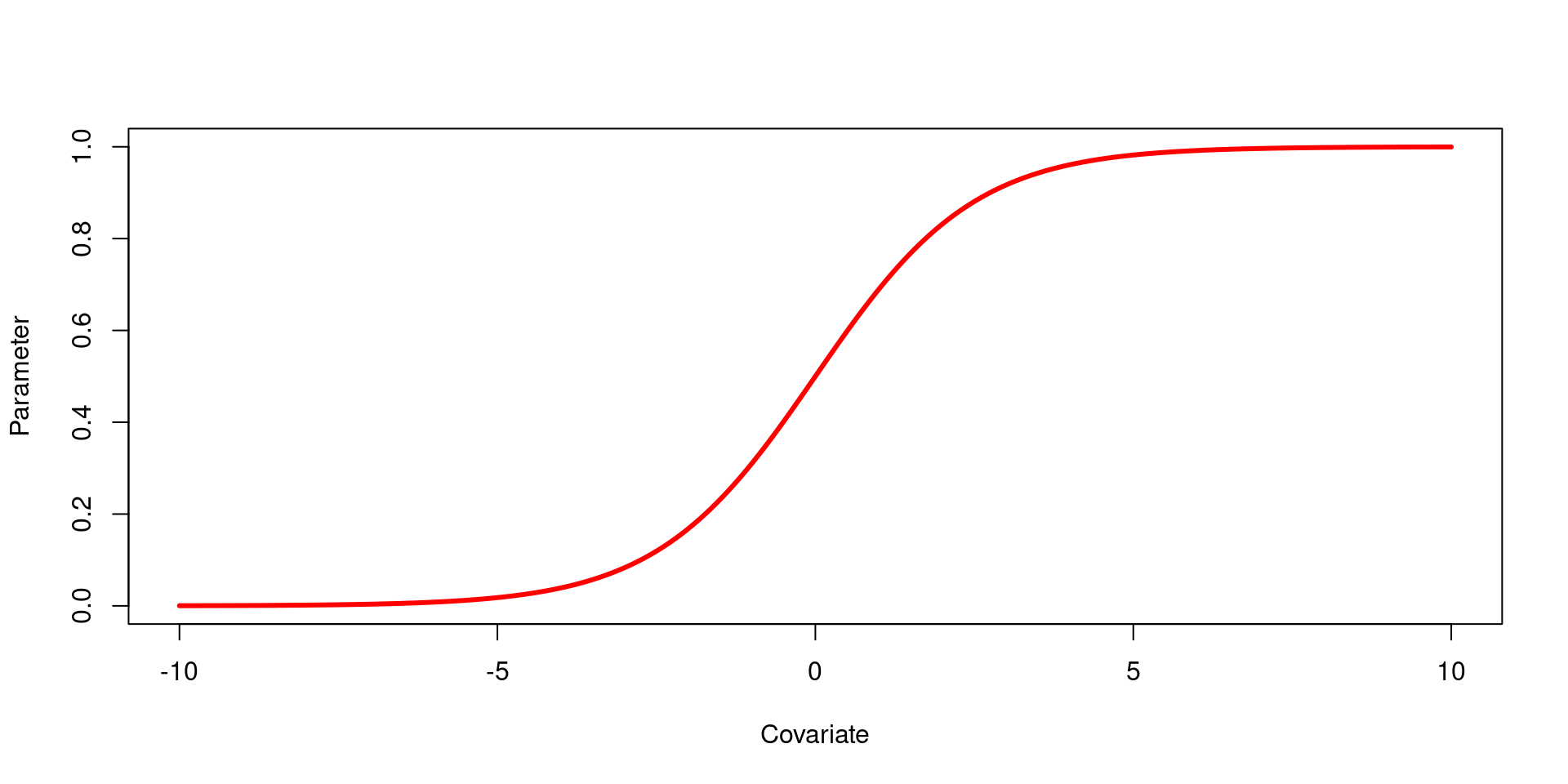
The logit link function creates an ‘S’-shaped relationship between a covariate1 and a parameter2, constraining the parameter to between zero and one
Logit link for coefficient = 0.8
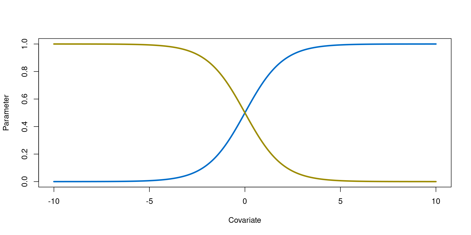
Coefficient sign
As with linear relationships, the sign of the coefficient indicates the direction of the relationship:
Positive coefficients (\(\beta\) = 1) indicate a positive correlation
Negative coefficients (\(\beta\) = -1) indicate a negative correlation
Logit link for positive and negative coefficients
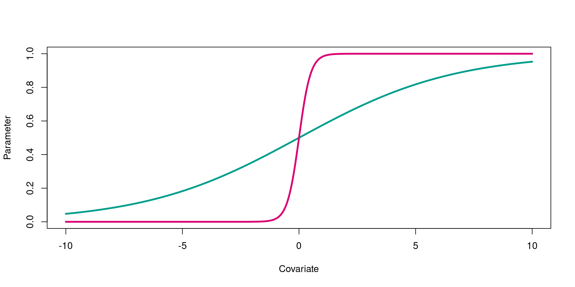
Coefficient magnitude
The magnitude (size) of the coefficient indicates how rapidly the parameter changes as the value of the covariate changes. For example, how sharply does detection (parameter) increase as you increase team size (covariate)
Small coefficients (\(\beta\) = 0.3) generate gentle logit curves
Large coefficients (\(\beta\) = 4) generate steep logit curves
Logit link for small and large positive coefficients
Ecological interpretation
💡 Let’s use these principles to help us understand our water deer results
hnLC_.
Call:
distsamp(formula = ~Landcover ~ 1, data = TruncUMF, keyfun = "halfnorm",
    output = "density", unitsOut = "ha")

Density:
 Estimate    SE     z   P(>|z|)
    -2.63 0.113 -23.3 1.89e-120

Detection:
                 Estimate    SE     z   P(>|z|)
(Intercept)          5.03 0.174 28.85 4.67e-183
LandcoverWetland    -1.29 0.176 -7.29  3.06e-13

AIC: 271.3911
The intercept of Density is negative - density is less than one deer per hectare
The intercept of Detection is positive - this is the coefficient for detectability in grassland
LandcoverWetland is negative - detectability in wetland is lower than in grassland, probably because the vegetation is taller in reedbeds
Calculate parameter values
We can use unmarked’s backTransform() function to generate density and detectability estimates from our models
We’re going to estimate density and detectability for our second best model, hnLC_DTC, so we can see the process for estimating density and detectability when they’re both influenced by covariates
Density and covariates
When estimating density or detectability from a model with covariates, we need to provide backTransform() with specific values of the covariates
Let’s investigate the effect of proximity to the coast on density by generating two estimates at different distances from the coast:
Density at 50m - close to the coast
Density at 500m - further from the coast
Remember covariate transformations!
Bear in mind that we rescaledDistToCoast from metres to kilometres, so we must provide distances to linearComb() in kilometres
Distances from the coast
Use covariate values in linearComb() inside backTransform()
The estimated densities are 0.064 animals per hectare (or 6 per square kilometre) 100m from the coast, and 0.064 animals/hectare (6 per square kilometre) 400m from the coast
This confirms our interpretation that DistToCoast has little influence - in fact, the difference is undetectable at these distances from the coast!
The overlapping confidence Intervals for these two density estimates are further proof that DistToCoast is not biologically meaningful:
DensDTC50_CI <-confint(DensDTC50)DensDTC50_CI
      0.025     0.975
 0.04001007 0.1037962
DensDTC500_CI <-confint(DensDTC500)DensDTC500_CI
      0.025     0.975
 0.04003884 0.1037585
The weight of evidence for our hnLC_DTC model is probably caused by how well the other parameters fit the data, and DistToCoast is incidental. We’ll dig further into this in the next module
Detectability and covariates
For detectability, we’ll create two contrasting scenarios:
Transects in grasslands 🌾
Transects in wetlands 💦
We’ll estimate detection probability separately for these two landcover classes
Backtransformed detection functions
Remember that back-transforming the estimate from a half-normal detection function gives us the half-normal standard deviation
This tells us the distance within which c. two-thirds of the water deer were sighted
Coefficients for categories
For qualitative covariates, the first category1 is the reference category
The intercept of our model equation is the reference category’s coefficient
For all other categories, R estimates a separate coefficient
The effect of a non-reference category is the intercept plus the category’s coefficient
This means a category’s coefficient shows its effect in relation to the reference category
In our water deer case-study, the reference category is Grassland🌾
Coefficients for categories in linearComb()
The first coefficient represents the intercept - the effect of our reference category
The second coefficient codes the category - set this to 0 for Grassland🌾 and 1 for Wetland💦
Detectability in grassland
First let’s backtransform our estimate for detectability in grassland🌾
Set coefficients to 1 for intercept and 1 for our alternative category, Wetland💦
3
Calculate detectability
Backtransformed linear combination(s) of Detection estimate(s)

 Estimate   SE LinComb (Intercept) LandcoverWetland
     41.9 3.99    3.74           1                1

Transformation: exp
The half-normal standard deviation in grassland is 152m
In contrast, the half-normal standard deviation in wetland is only 42m
➡️ Detectability is much lower in wetland
Confidence intervals: Detection
Strengthen your understanding of the difference in detectability between wetland and grassland by assessing the confidence intervals for our estimates
Adapt the code from earlier in this exercise to generate and view confidence intervals
Grassland CI
    0.025    0.975
 107.0287 215.7588
Wetland CI
    0.025    0.975
 34.80466 50.53005
Non-overlapping CIs
Note how the confidence intervals for the two landcover classes do not overlap. This provides further support to our conclusion that detectability varies between grassland and wetland
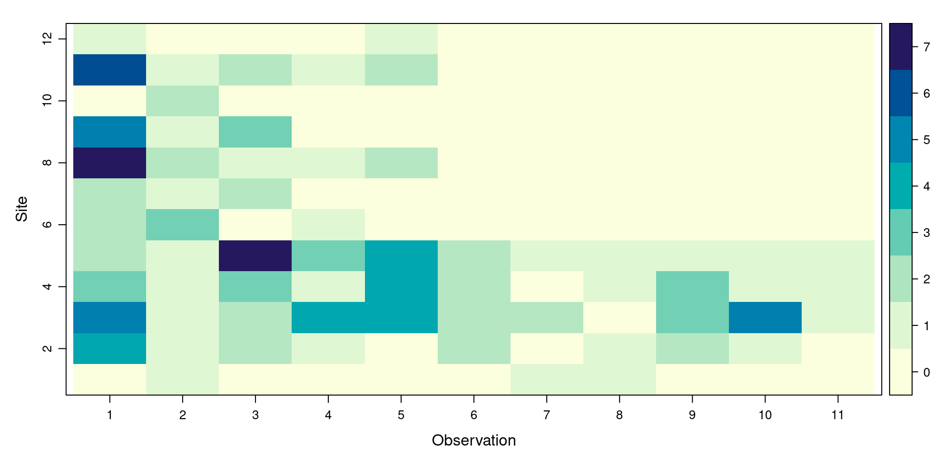
Review data and conclusions
Remind yourself of which landcover class each transect was surveyed in, and revisit the illustration of sightings at different distances from the transect
❓
Do the field observations suggest that your statistical results are correct or false?
TruncUMF@siteCovs
   Landcover Team DistToCoast
1  Grassland    A         230
2  Grassland    B         330
3  Grassland    B         480
4  Grassland    B         190
5  Grassland    A         430
6    Wetland    A         230
7    Wetland    B         270
8    Wetland    A         320
9    Wetland    B         120
10   Wetland    B         160
11   Wetland    A         150
12   Wetland    A         260