Prepare covariates
Parameter estimation
As you know, distance sampling analysis involves estimating the parameter values which are most likely, given our field observations
Parameters include:
- Density
- Shape of the detection function
- Coefficients of covariates affecting density and detectability
The resulting equations can be complex, and finding the correct parameter values requires computational algorithms
Transform covariates before analysis
To increase the chance that R’s algorithms will converge on suitable estimates for all the parameters you’re interested in, we transform covariates before analysis
We want all transformed covariates to lie in a similar range, rather than being orders of magnitude different from each other
This can be done by scaling or standardising
Transform continuous covariates
If your covariate values are large, or vary by an order of magnitude or more, convert them to a reduced scale before analysis
Aim to bring them into the range of -1 to +1, or zero to 2-3
Choose a scaling method that offers you an intuitive understanding of the data. For example:
- Convert percentages (0 to 100) to proportions (0 to 1), e.g. canopy cover 🌳
- Divide large numbers by a constant so that the scale is still meaningful but the values lie closer to 1. For example, convert altitude from metres to km above sea level
- Scale large numbers to lie between 0 and 1 by dividing them by their maximum value, or by an appropriate order of magnitude. For example, divide distances in the range of 10s of km by 100
- Standardise your data by subtracting the mean and dividing by the standard deviation. This creates z-scores (mean = 0, SD = 1) which can be interpreted as how each individual transect compares to the average value over all transects
Convert categories to factors
Let’s make sure R recognises our Landcover and Team covariates are categorical, using factor()
Skip this step if you already did it at the end of the previous exercise
Combine detections and covariates
Re-create our distance sampling unmarked frame (UMF), this time including transect covariates:
1TruncUMF <- unmarkedFrameDS(
2    y = as.matrix(TruncyDat),
3    siteCovs = Covs,
4    dist.breaks = TruncDistBins,
5 tlength = TransectLengths$Length, survey = "line", unitsIn = "m")- 1
- Overwrite our original UMF
- 2
-
TruncyData is our earlier output from
formatDistData() - 3
- Specify our transect covariates
- 4
- Specify truncated distance bins
- 5
- Provide transect lengths, type of survey and distance measurement units as before
Visual checks: Summary
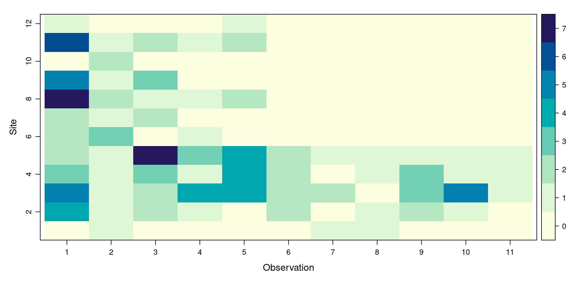
Do a quick visual check to see everything looks okay:
unmarkedFrameDS Object

line-transect survey design
Distance class cutpoints (m):  0 20 40 60 80 100 120 140 160 180 200 220

12 sites
Maximum number of distance classes per site: 11
Mean number of distance classes per site: 11
Sites with at least one detection: 12

Tabulation of y observations:
 0  1  2  3  4  5  6  7
68 29 17  7  5  3  1  2

Site-level covariates:
     Landcover Team   DistToCoast
 Grassland:5   A:6   Min.   :120.0
 Wetland  :7   B:6   1st Qu.:182.5
                     Median :245.0
                     Mean   :264.2
                     3rd Qu.:322.5
                     Max.   :480.0
Visual checks: Plot
Decide on transformations
We need to:
- Decide which re-scaling approach to apply to our continuous covariates, to bring them to a scale close to 0-1
- Calculate the new covariate values
Rescale within the UMF
We are going to rescale the covariates stored in our new TruncUMF object, rather than re-scaling the original data
Examine the summary a few slides back to refresh your memory of the format and distribution of site covariates
Which covariates do we need to transform?
Re-scale continuous covariates
The levels of both the nominal variables (Landcover and Team) will be coded by R as 1 and 2 during analysis, so it’s not necessary to rescale them
DistToCoast requires re-scaling because it ranges from 120m to 480m
Re-scale DistToCoast by converting from metres to kilometres:
Check your calculation worked by using summary() to re-examine the covariates in TruncUMF