Detection functions

How can we estimate detectability?

To estimate detectability, we need to understand how our ability to detect an animal varies depending on how far it is from the transect line

It’s likely that animals or sign further away from the line are less likely to be spotted

In other words…

Probability of detection decreases with distance from the transect

If we plot Probability of detection on the y axis against Distance from the transect line on the x axis, we would expect a line that slopes down to the right

This line¹ is called the detection function

1. or rather, the equation relating detection probability to distance, from which our line is drawn

Gathering data

1. You (eye symbol) walk along the transect (blue) and see a deer
2. You estimate the distance from you to the deer (radial distance; yellow)
3. You use your compass to record the bearing to the deer
4. This bearing later allows you to calculate the angle between the transect and the deer (θ; brown angle)
5. During analysis, radial distance & angle are converted into perpendicular distance¹ (green)

1. Perpendicular distance: Shortest distance between transect and deer

Frequency histogram

As you walk further and spot more deer, you build up a graph of how many were recorded at different distances from the transect

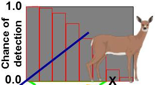
• The x axis is perpendicular distance from the transect
• The y axis is number of sightings, which equates to probability of detection
• The frequency histogram (red bars) indicate the number of deer sighted at different distances from the transect, equivalent to chance of detection

The detection function

As you can see, the histogram tails off as deer are further from the transect

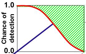
We can fit a mathematical model to the histogram bars, describing the shape of this decline in observations

This mathematical model (red curve on the graph) is the detection function

Use the detection function

1. You saw all the animals under the detection function (red curved line)
2. You know that the number of animals doesn’t actually decline further away from the line - it’s simply your ability to detect them that drops with distance
3. So you can assume that there are also animals that you did not see (green shaded area above the red detection function)
4. This green area shows us the proportion of animals within our surveyed area that we did not observe

Effective strip width

Effective strip width: the distance at which the number of animals you detected beyond that distance is equal to the number of animals you failed to detect within that distance

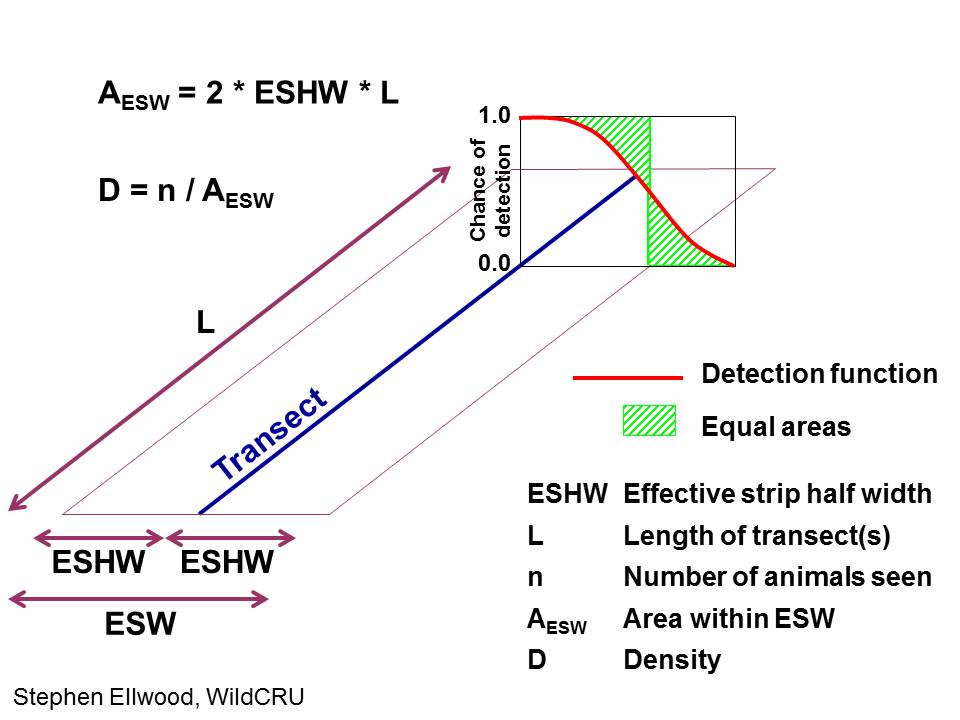
• The two green shaded areas are equal in size
• You can multiply the transect length by the ESW to calculate the area surveyed
• Dividing the number of deer that you saw by this area gives you your estimate of deer density

Maximise detectability

Even if we’re estimating detectability, it’s important to try and maximise the chance of detecting animals:

1. The species that we work on are often at low density, elusive, or declining
2. We need a sufficiently large sample size¹ to be confident that we’re modelling the shape of the detection function correctly
3. High detectability gives us more accurate density estimates

We return to this idea in the Analysis and Survey design courses

1. Sample size: distance walked ~ number of individuals recorded