Case study: Black crested gibbons

Throughout this course, we encourage you to use your own field data so you can immediately apply what you’re learning. However, we know that it can be easier to start with a simplified dataset that matches what your fellow learners are using, so we also provide data from a case-study of the Critically Endangered western black crested gibbon, Nomascus concolor in Chế Tạo Nature Reserve in northern Vietnam

Gibbons are arboreal apes dependent on continuous forest canopy. They live in monogamous family groups composed of a breeding pair and usually 1-2 infants/juveniles. Nomascus concolor was thought to be extinct in Vietnam until it was rediscovered in 2000. See the IUCN Redlist page on black-crested gibbons for more information on their ecology and conservation.

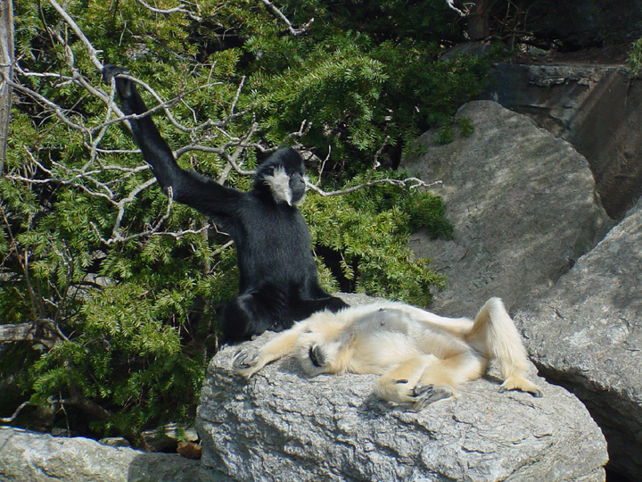
Western black crested gibbon pair¹

Your first QGIS project

Let’s start your first QGIS project! We’ll add gibbon sightings from our survey, and distribution information from the IUCN Redlist record for this species²

First you’ll need to download the gibbon sightings. Clicking on the links below will either open a ‘Download’ pop-up in your browser, asking you where to save the files, or automatically download them to the usual location on your computer, depending on your web browser settings

1. First create a new folder for your first GIS project, ready to store the gibbon sightings
2. Download NomascusConcolor_Distribution.zip
3. Unzip the gibbon distribution files into your folder
4. Download GibbonSightings_Survey1.geojson
   1. If you’re having difficulty downloading the .geojson file, try downloading and unzipping this .zip archive instead: GibbonSightings_Survey1.zip

Note how the two datasets are in different file formats. The gibbon sightings are a single .geojson file, while the species distribution dataset is an ESRI shapefile, composed of many separate files with different file extensions: .shp, .dbf etc

Let’s add the distribution data to QGIS:

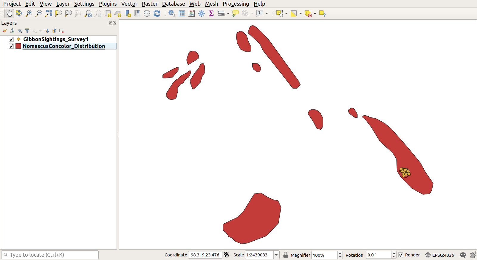
1. In QGIS, click on the Layer menu > Add Layer > Add Vector Layer...
2. Choose the source file by clicking the […] button and finding NomascusConcolor_Distribution.shp - note that it’s the file ending in .SHP that you need to add to QGIS. You should several polygons of different sizes and shapes added to your map, which represent this species’ distribution

Now we’ll add the gibbon sightings:

1. Repeat the same process using Add Vector Layer... to add GibbonSightings_Survey1.geojson
2. Click Add and Close. You should see the points clustered in the right-hand polygon on your QGIS map view - we’ll zoom in and inspect them shortly
3. Save your project in the same folder as the gibbon sightings file: Project > Save

Your new project should look like this:

---

---